Vacuum Tube Parameter Identification Using Computer Methods

MITHAT F. KONAR
Biro Technology
http://www.birotechnology.com

A method for identifying vacuum tube SPICE model parameters using computerized optimization is presented. The method is applied to a computationally efficient triode model for three different triodes and the results compared to the reference data and 3/2 power-law models.

Introduction
If any evidence is required of audio's seemingly eternal vacuum tube renaissance, one need only look at the various attempts that have recently been made to use SPICE and its derivatives for vacuum tube audio design [1] - [7]. While few will assert that these models have reached a state of maturity, they nonetheless offer the tube equipment designer many powerful benefits that have previously only been available to designers working with solid-state devices.

In this paper we present a method for determining vacuum tube SPICE model parameters using computerized optimization. The parameters of interest in the work presented are those which affect the characteristic plate curves for vacuum tube triodes; interelectrode capacitances, heater characteristics, grid current, influences of additional grids, etc. will not be considered further.

A review of the models used in this paper
Fundamental vacuum tube models (e.g., those presented by Intusoft [1], Reynolds [2] and Leach [6]) are based on direct implementations of the idealized "3/2 power law" for current flow in an ideal triode:

, (1)

where i_p is the instantaneous plate current, v_G is the instantaneous grid voltage, v_P is the instantaneous plate voltage, µ is the tube's amplification factor, and K_G is a constant of proportionality called the perveance. (In this and all subsequent relations it is assumed that the cathode is at ground potential. In addition, the above and subsequent relations are valid only when their respective quantities between the parenthesis are positive. When this quantity is negative, no plate current will flow.)

Expanding on the 3/2 power law, Koren presented phenomenological models for vacuum tube triodes and pentodes which were shown to effectively model the behavior of tubes over a wide range of plate voltages and currents [4]. To model triodes, Koren used the following equations:

(2a)

and

.(2b)

Here µ and k_G1 are essentially the amplification factor and twice the inverse of the perveance from the 3/2 power law, x is the exponent in the 3/2 power law, and k_P and k_VB control the nature of the "bending" of the curves near cutoff. (The (1+sgn(E1)) portion of equation (2b) forces the plate current to zero when E1 is negative.)

Koren [4] states his approach "takes advantage of the fact that log(1+exp(x)) approaches x when x>>1, and 0 for x<<1." Thus, at high plate currents this model behaves very much as the 3/2 power law--with the exception that the 3/2 exponent is now treated as a variable parameter. However, at low plate currents, the log(1+exp(x)) relationship results in behavior that effectively mimics the behavior of real-world tubes at low currents. In addition, these performance improvements are achieved with relatively low computational complexity and with only three additional parameters.

Parameter identification using analytic methods
A primary concern associated with using any model is determining an appropriate set of parameters which results in the desired behavior. Since there are only two unknown parameters in the 3/2 power law, it is a relatively simple matter to solve for them using two data points. Letting i_p1, v_G1, and v_P1 represent the first data point and i_p2, v_G2, and v_P2 the second, we next define:

.(3)

Solving for µ using two data points yields:

(4)

and

.(5)

Since the 3/2 power law isn't 100% accurate, the values resulting from the computations above will depend somewhat on the selected data points. More-or-less acceptable results typically ensue if the first point is taken at zero grid bias and relatively high plate current and the second at a fairly low grid voltage and relatively low plate current--taking care to avoid the region where the tube enters cutoff.

Unfortunately, the simple parameter identification method used above becomes unmanageable in the case of Koren's (and most others') triode models because of the large number of parameters involved--and hence the large number of equations to simultaneously solve. To find parameters for Koren's model, its inventor suggests using an iterative method starting with parameters appropriate for the 3/2 power law [4]. Unfortunately, the tedium and uncertainty of open-ended iterations over five (or more in the case of other models) variables makes this a rather unappealing prospect.

Computer-based optimization applied to parameter identification
The solution explored in this paper is the use of computer-based optimization methods to identify model parameters. Such a solution was implemented using MATLAB--a multi-platform numeric computation and visualization software package [8]. The primary advantages to using MATLAB for development of the method include transportability of code and rapidity of development.

At its simplest, a numeric computation and visualization environment can be used to easily plot a model's plate characteristics and compare those curves against a set of reference data points. This can speed up an iterative parameter hunt considerably. However, the real power of a tool such as MATLAB lies in the ability to automatically find model parameters using pre-programmed optimizing algorithms. To this end, we have implemented an extensible set of MATLAB scripts and functions (refereed to as m-files) and have successfully used them to determine model parameters for a number of triodes. The code was designed such that wherever possible speed is maximized and specificity minimized. Thus, any of a number of user-implemented tube models or optimizing functions found in MATLAB's Optimization Toolbox can be used with very little code modification.

Within the m-files, model parameters are found by minimization of an error function. The error function can be selected to return the mean fractional error over all reference points or the RMS fractional error. Because most minimization algorithms do not constrain variables and because negative values for parameters used in the Koren model (and many others) are unacceptable, logarithmic transformation of variables was used to constrain parameters to positive values without losing the ability to use unconstrained optimizers. While this increases the calculation burden, it prevents the optimizer from converging on unacceptable final parameters.

Discussion
For the work presented in this paper, MATLAB's fmins() function was used as the error minimizer because it is bundled with the version of the Optimization Toolbox that ships with the student version of MATLAB. Unfortunately, fmins() is exceedingly slow owing to its use of a simplex minimization algorithm. Thus, depending on the speed of the computer, how close the initial parameters are to the final parameters, and operator patience, the time it takes to converge on an optimal parameter set may be annoyingly long.

Another characteristic of the fmins() function (and something that is typical of minimization algorithms in general) is that it will find only a local minimum of a function and not necessarily the function's absolute minimum. Thus, it is important to define the initial parameters as close to the expected final parameters as possible or to perform numerous optimizations beginning from different points.

For the optimizations presented below, initial parameter values were set as follows: µ as calculated for the 3/2 power law, k_G1 to 1/(2K_G) (where K_G again comes from the 3/2 power law model), x to 1.5, and k_P and k_VB to 500. After some experimentation, it was found that reference data consisting of approximately 50 carefully selected points was, in a sense, ideal for the triodes investigated. Fewer points resulted in rising error while additional points yielded little improvement.

Given the somewhat lengthy time it takes for the MATLAB m-files to converge and the burden of preparing a data file with 50 or so points, one might feel that this method merely replaces one kind of tedium for another. While this may be a legitimate sentiment, it should be kept in mind that the method presented here represents more of a closed solution than the hunt-and-peck of manual iteration.

Examples
To determine the effectiveness of the above method, it was used to find the parameters for three small-signal triodes: 6DJ8, 12AT7, and 5842. The resulting plate characteristics for the 6DJ8 appear in Fig. 1 and those for the 12AT7 and 5842 appear in Figs. 2 and 3. The parameters for all three are listed in Table 1. (Note: Reference data for the 6DJ8 and 12AT7 tubes were taken from third-party curves of actual tubes [9] while the data for the 5842 were taken from manufacturer's published data [10].) To compare models, the "two-point" method was used to find the parameters for the same three triodes using the 3/2 power law. These results appear in Figs. 4, 5, and 6 and Table 2.

The performance of the Koren model using parameters determined by computerized optimization yields a worst-case mean error of 6.5% for the reference points used. In general it performs with at least a five-fold reduction in error compared to the 3/2 power law models, and improvements can be seen throughout the operational range of the tube--not just in the cutoff region as may be expected. It is interesting to note the significant divergence from the 3/2 exponent for the 5842 tube. This is likely the result of the somewhat unconventional grid construction used in this tube; however, it may also be due to inaccurate performance data reported in the databooks.

Conclusion
There is no reason that the optimization-based parameter identification method presented in this paper cannot be extended to other vacuum tube models--including pentode and other triode models. However, other models with which the author is aware (apart from those which are direct implementations of the 3/2 power law) all use more than the five parameters used in Koren's triode model. Since optimizing for five parameters has been demonstrated to be inconveniently time consuming using the m-files used in this paper, to optimize over a larger number of parameters will require faster optimization routines and/or a process implemented in a compileable language. However, the results presented herein indicate that doing so will provide a highly effective means of parameter identification.

REFERENCES

[1] "A SPICE Model For Vacuum Tubes," Intusoft Newsletter, (1989 Feb.).

[2] S. Reynolds, "Vacuum-Tube Models for PSpice Simulations," Glass Audio, vol. 5, no. 4, pp. 17-23 (1993).

[3] "Modeling Vacuum Tubes: Parts I and II," Intusoft Newsletter, (1994 Feb. and Mar.).

[4] N. Koren, "Improved Vacuum-Tube Models for SPICE Simulations," Glass Audio, vol. 8, no. 5, pp. 18-27+ (1996).

[5] W. Sjursen, "Improved SPICE Model For Triode Vacuum Tubes," J. Audio Eng. Soc., vol. 45, pp. 1082-1088 (1997 Dec.).

[6] W. M. Leach, Jr., "SPICE Models for Vacuum-Tube Amplifiers," J. Audio Eng. Soc., vol. 43, pp. 117-126 (1995 Mar.).

[7] J. Maillet, "Algebraic Technique For Modeling Triodes," Glass Audio, vol. 10, no. 2, pp. 2-9 (1998).

[8] MATLAB, The MathWorks, Inc., Natick, MA.

[9] Audiomatica WWW site, http://www.mclink.it/com/audiomatica/sofia/.

[10] currently unidentified source.

TABLES and FIGURES

TABLE 1: Parameters for Koren's model determined by computerized optimization.

tube	µ	x	kG1	kP	kVB	mean fractional error
6DJ8	35.7	1.35	274	305	310	5.3%
12AT7	58.5	1.23	659	267	1849	3.7%
5842	42.4	2.21	393	629	446	6.5%

TABLE 2: Parameters calculated for 3/2 power law model using "two-point" method.

tube	µ	KG	mean fractional error
6DJ8	33.2	6.29e-3	29%
12AT7	53.0	2.01e-3	23%
5842	44.8	10.3e-3	32%

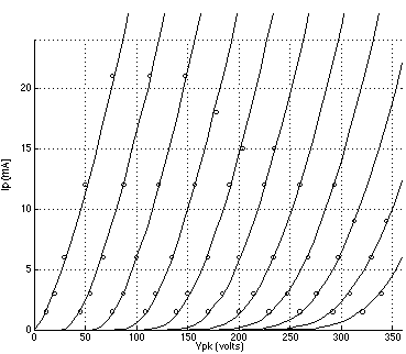
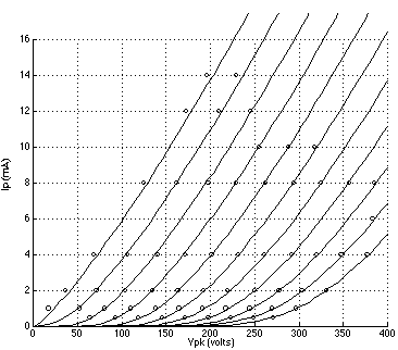
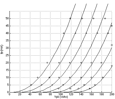
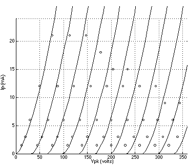
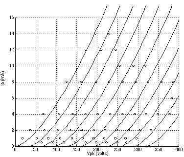
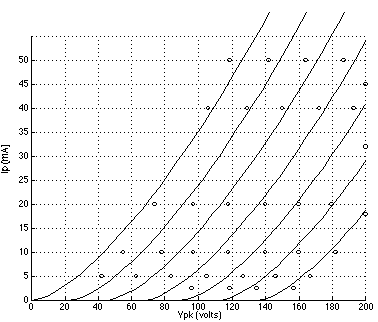
FIGURE 1: 6DJ8 plate curves using Koren's model with parameters listed in TABLE 1; grid voltage = 0 to -10 volts. (Reference data points are indicated by circles.)

FIGURE 2: 12AT7 plate curves using Koren's model with parameters listed in TABLE 1; grid voltage = 0 to -6 volts. (Reference data points are indicated by circles.)

FIGURE 3: 5842 plate curves using Koren's model with parameters listed in TABLE 1; grid voltage = 0 to -3 volts. (Reference data points are indicated by circles.)

FIGURE 4: 6DJ8 plate curves using a 3/2 power law model with parameters listed in TABLE 2; grid voltage = 0 to -10 volts. (Reference data points are indicated by circles.)

FIGURE 5: 12AT7 plate curves using the 3/2 power law model.with parameters listed in TABLE 2; grid voltage = 0 to -6 volts. (Reference data points are indicated by circles.)

FIGURE 6: 5842 plate curves using the 3/2 power law model with parameters listed in TABLE 2; grid voltage = 0 to -3 volts. (Reference data points are indicated by circles.)

APPENDIX

PSpice files using Koren's model and parameters found using the above method are available at the following links:
6DJ8/ECC88
6SN7
12AT7/ECC81
12AU7/ECC82
5842/417A

r 0.05 26 Dec 2003

Site copyright ©2005 Biro Technology–all rights reserved